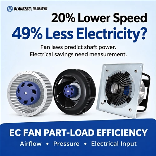
Does a 20% EC Fan Speed Reduction Really Cut Electricity Use by 49%?
Fan laws, shaft power and electrical input: a practical guide to EC fan efficiency and measured part-load savings in air handling units.
For AHU manufacturers, retrofit teams and data-center cooling operators, the distinction changes equipment selection and payback calculations. An EC fan can offer controllable airflow, but a speed command alone does not establish the power drawn from the supply. This guide connects centrifugal fan power calculation with a measurement plan that procurement and commissioning teams can review.

A speed reduction changes shaft demand. Electrical savings depend on the complete operating point and measurement boundary.
In this guide1. Which power belongs in an EC fan efficiency calculation?
Begin by naming the quantity, units and measurement location. Rated power describes a declared rating under stated conditions; it is not a reading of current consumption. A motor nameplate may state rated mechanical output, while a fan datasheet may specify electrical input. Read the definition before comparing numbers carrying the same "W" label.
| Quantity | What it describes | Use in the project |
|---|---|---|
| Rated power | A declared motor or fan rating with specified conditions and a defined input or output basis. | Check suitability and limits; do not substitute it for measured consumption. |
| Fan shaft power | Mechanical power delivered to the impeller shaft. | Use with aerodynamic similarity calculations and shaft-to-air efficiency. |
| Electrical input power | Real power crossing a specified electrical boundary. | Use for energy calculations, including the loads inside that boundary. |
Air power provides another useful reference: airflow multiplied by a consistently defined pressure rise. For a total-pressure calculation, Q in m3/s multiplied by fan total pressure in Pa gives watts. Dividing that air power by fan shaft power gives total fan efficiency; dividing it by electrical input gives total wire-to-air efficiency. Static-pressure efficiency uses a different numerator and must be identified separately.
A centrifugal fan power calculation therefore needs more than airflow and a motor rating. It needs pressure type, fan efficiency at the duty point and, when estimating electricity, the motor/controller conversion efficiency. A direct-drive arrangement removes a belt transmission from the power chain; it does not remove electrical or aerodynamic losses.
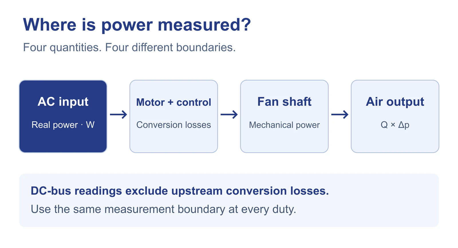
The AC input, internal DC bus, shaft and air are different accounting boundaries. The simplified drive layout varies by product. On small screens, swipe horizontally to inspect the full diagram.
AMCA Publication 211-22, Annex H, treats the fan and motor/controller power-drive system separately when deriving electrical input from component tests. It includes EC motor arrangements and uses efficiencies at the required speed and load, rather than nominal nameplate efficiency. This supports requesting a duty-specific power map; it does not certify any particular product shown here. Source: AMCA 211-22, Annex H.
2. When do fan laws support the "49%" calculation?
For the same fan diameter and geometry, comparable operating points and approximately unchanged aerodynamic efficiency, the familiar speed relationships are:
r = N2 / N1
Q2 / Q1 ≈ r
Δp2 / Δp1 ≈ (ρ2 / ρ1) × r2
Pshaft,2 / Pshaft,1 ≈ (ρ2 / ρ1) × r3
N is rotational speed, Q is volume airflow and ρ is air density. At unchanged density and r = 0.80, airflow becomes approximately 80%, pressure 64%, and shaft power 51.2% of their reference values. The corresponding shaft-power reduction is 100% − 51.2% = 48.8%, conventionally rounded to 49%.
These are corresponding points on similar fan characteristics. An installed AHU follows them only if its system behavior permits that movement. A fixed resistance dominated by approximately quadratic flow losses, without a significant fixed pressure component, is a useful approximation. Damper changes, filter loading, coil conditions, fan staging and pressure-reset sequences can change the operating path.
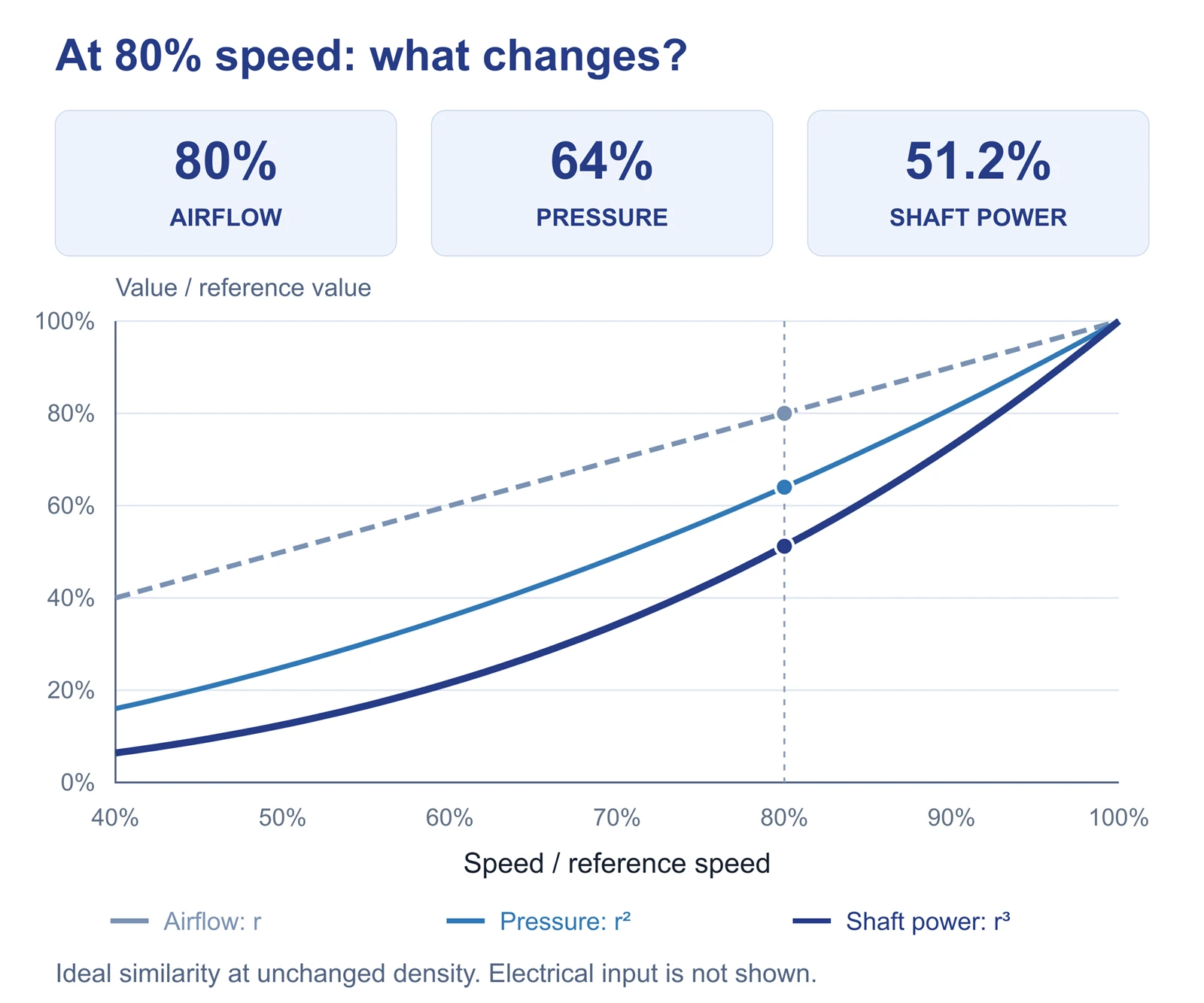
Calculated similarity relationships, not measured Blauberg performance. The shaft-power curve is not an electrical-input curve. On small screens, swipe horizontally to inspect the full diagram.
Also confirm density and installation geometry. Inlet restrictions, outlet obstructions or changed clearances can invalidate a simple comparison. At low speeds, changing Reynolds number, instability or altered efficiency may reduce the accuracy of similarity scaling. Use manufacturer limits and curves to define the useful range. The U.S. Department of Energy's fan-system sourcebook provides the broader system-selection context. Source: Improving Fan System Performance.
Reducing airflow is only an energy measure when the lower delivery still meets the required ventilation or cooling service. A lower meter reading caused by insufficient airflow is not evidence of improved efficiency at equivalent service.
3. Why does EC fan electrical input depart from the cube law?
For a direct-drive fan, a useful accounting model is Pelectrical = Pshaft / ηmotor+controller + Paux. Here the combined efficiency covers the declared motor/controller boundary, including its losses. Paux contains only additional loads outside that efficiency definition but inside the selected meter boundary. Counting the same electronics in both terms would overstate consumption.
Motor copper and magnetic losses, switching losses, bearing losses and control consumption do not all vary with the same exponent. Their relative contributions change with speed, torque, temperature and operating mode. Some consumption can remain at low load or in standby. Neither a fixed loss percentage nor a universal electrical-power exponent should be assumed for every EC fan.
EC fan cube law vs electrical input: what does a worked example show?
Assume 1.000 kW shaft power at the reference point and 0.512 kW at 80% speed. Now assume combined motor/controller efficiencies of 90% and 80%, respectively, plus 0.020 kW of separately counted auxiliary consumption at both points.
| Illustrative quantity | Reference speed | 80% speed |
|---|---|---|
| Shaft power | 1.000 kW | 0.512 kW |
| Assumed motor/controller efficiency | 90% | 80% |
| Separately counted auxiliary load | 0.020 kW | 0.020 kW |
| Calculated electrical input | 1.131 kW | 0.660 kW |
| Reduction from reference | - | 48.8% shaft; approximately 41.7% electrical |
These are invented teaching inputs, not typical efficiencies, product test results or a savings forecast. Different efficiency maps and auxiliary loads produce different results. The example establishes why electrical input needs its own evidence.
What changes under constant-static-pressure control?
An AHU controller may hold pressure at a duct sensor while terminal dampers move. That sensor pressure is not necessarily the fan's total pressure rise. The effective resistance seen by the fan changes, so measured airflow need not fall in direct proportion to speed. If pressure across a defined boundary were actually constant, its air power Q × Δp would vary linearly with airflow, not cubically. This observation still does not establish a universal speed-to-electricity relationship.
The October 2026 SKW EnergyOS article reports DC-bus readings from one EC fan and identifies supply-voltage interference at lower-speed points. It is a useful case-specific observation, not a Blauberg test or a general exponent. A DC-bus measurement also excludes upstream conversion losses and any loads outside that bus boundary; it cannot simply be equated to grid input. Source: SKW EnergyOS, 10 October 2026.
CloudAir's October article similarly distinguishes shaft power from supply-side input. Its illustrative efficiency assumptions should not be transferred to a selected EC plug fan. Source: CloudAir, 26 October 2026.
Which centrifugal fan models should you review?
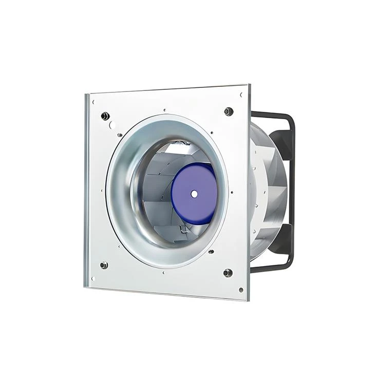
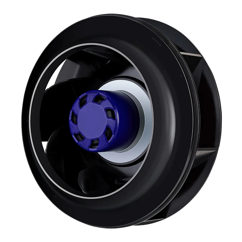
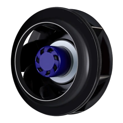
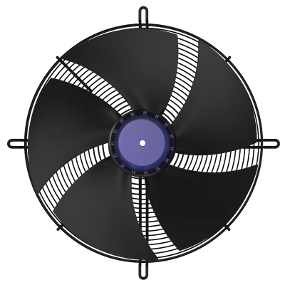
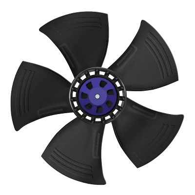
Blauberg GC-B310E-EC-05 310 mm EC Plug Fan
310 mm EC plug fan. Review the published curve and electrical input at your duty.
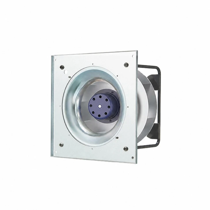
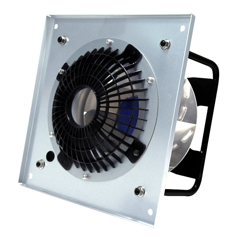
Blauberg GK-B310E-EC-05 310 mm EC Plug Fan
310 mm EC plug fan. Check the exact supply, mounting and control configuration.
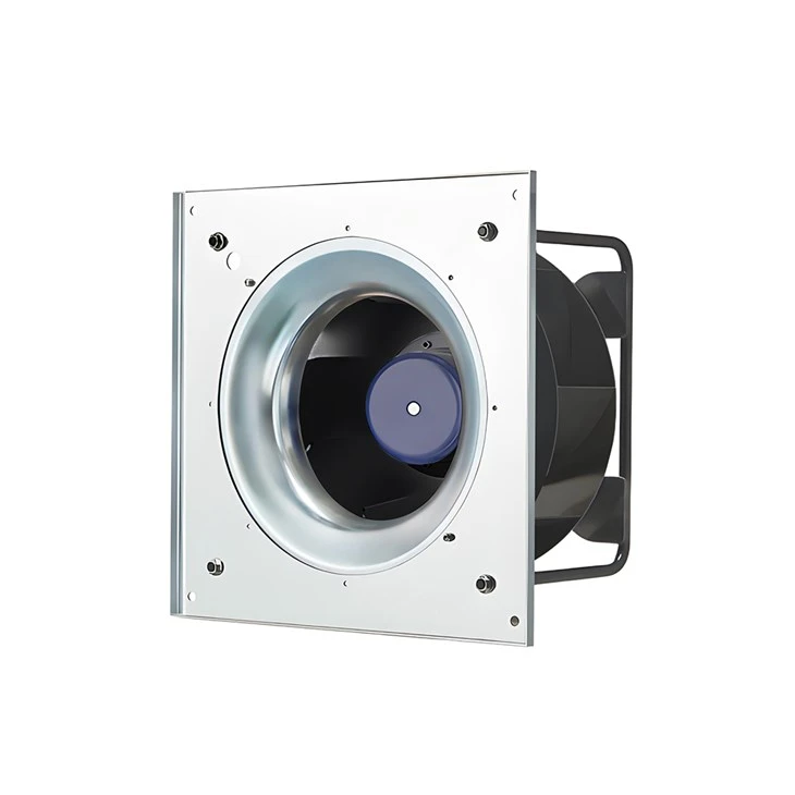
Blauberg GC-B310C-EC-F05 310 mm EC Plug Fan
310 mm EC plug fan. Compare the required airflow and pressure with its curve.
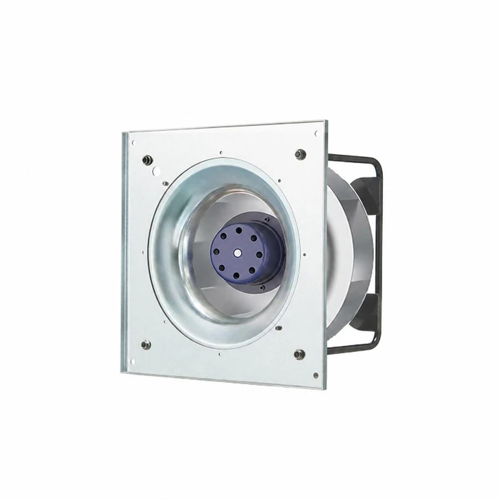
Blauberg GK-B400E-EC-05 400 mm EC Plug Fan
400 mm EC plug fan. Request low-, medium- and high-duty electrical-input data.
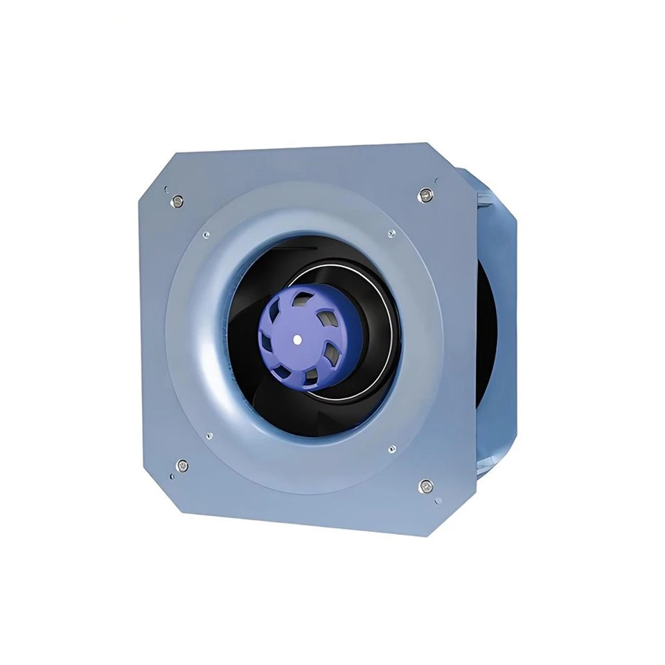
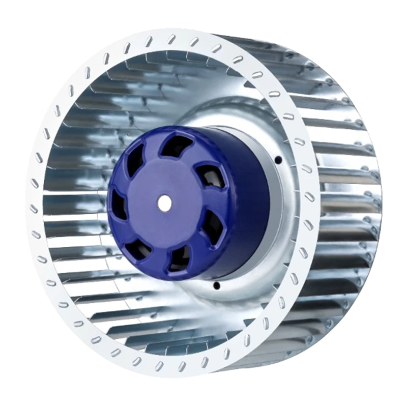
Blauberg GL-B220C-EC-M0 220 mm EC Fan
EC centrifugal fan. Verify the installation, supply and selected operating point.

Blauberg GY-B450E-EC-A5 450 mm EC Plug Fan
Backward-curved EC plug fan. Check the complete installed duty before selection.

Blauberg BL-B250D-EC-F05 250 mm EC Centrifugal Fan
Backward centrifugal fan. Review model-specific airflow, pressure and controls.
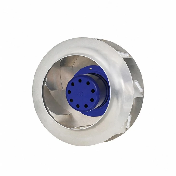
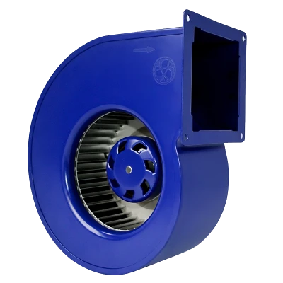
Blauberg 500 mm EC Backward-Curved Centrifugal Fan
500 mm EC fan range. Confirm the supply variant and part-load input power.
Review the linked model data at the required duty. The illustrative savings in this article are not ratings for these products.
4. How should AHU fan part-load power measurement be organized?
Start with low, medium and high duties representing the intended operating envelope. Approximately 60%, 80% and 100% of a defined reference speed can be a planning example, provided all are permitted and meet the test purpose. They are not mandatory test speeds. Include more points where controls change mode, fans switch on or off, or the power relationship bends.
Separate two questions: a controlled speed sweep checks behavior under deliberately fixed conditions, while a commissioning test checks performance with the intended automatic control sequence. Label the dataset accordingly. For an AHU plug fan, mixing those two datasets can make a controller response look like a motor-efficiency effect.

Illustrative fan-array arrangement. Record the active fan count and control mode, and verify each operating state at the same electrical measurement boundary.
| Record at every point | Minimum context |
|---|---|
| Actual speed and airflow | rpm; actual m3/s or m3/h; sensor locations and airflow method; distinguish actual from standardized volume. |
| Pressure and density | Static or total pressure, tap locations, temperature, atmospheric pressure and relevant humidity information. |
| Electrical input | Real W or kW; meter boundary, supply voltage, phase arrangement, instrument accuracy and included auxiliary loads. |
| Controls and installation | Setpoint, actual command, sensor position, damper/filter state, active fan count and software configuration. |
| Time and stability | Warm-up and settling duration, averaging window, timestamps, repeat readings, variability and abnormal events. |
For electricity-saving verification, normally measure upstream of the complete fan drive at its AC supply, with clearly identified shared auxiliaries. Use a suitable real-power analyzer for the supply and waveform. Multiplying RMS voltage by RMS current gives apparent power for a single-phase circuit, not necessarily real watts; distorted current makes assumptions especially unreliable.
Internal DC-bus telemetry can support diagnostics if its accuracy, averaging and boundary are documented. Even there, the average of instantaneous voltage times current can differ from the product of separately averaged readings. Controller-reported power may be measured or estimated: obtain its definition and cross-check against the project reference meter.
Agree stability criteria before testing instead of declaring every point settled after an arbitrary number of minutes. Observe the control response and motor temperature, average over a representative stable window, and repeat selected points in both directions. Flag voltage dips, pressure hunting and changing dampers. Retain excluded readings with an explanation so the final curve remains traceable.
Record measurement uncertainty alongside the result. Three points are an initial check, not proof of an entire performance map. Where the expected difference is close to instrument and operating variability, improve the measurement or report the uncertainty rather than presenting a precise saving.
5. How do measured power points become annual energy savings?
A local power-law fit can help interpolate a stable operating regime. Between two comparable positive-speed, positive-power points, n = ln(P2/P1) / ln(N2/N1). Label whether P is shaft, DC-bus or AC input power. Check additional points and residuals before using the fit; a closely spaced speed pair makes the exponent sensitive to measurement noise.
Do not force a curve through zero when there is standby consumption. A model with an offset may be more suitable, but three points alone can hide overfitting. Fan staging or control-mode changes generally require separate operating regions. Interpolate inside the validated envelope and obtain more evidence before extending outside it.
Annual electrical energy is the sum of input power multiplied by time in each operating bin: E = Σ(Pi × hi). The following arithmetic example assumes identical delivered service within each paired baseline/proposed bin and zero fan-system consumption during the off period.
| Illustrative service bin | Hours/year | Baseline kW | Proposed kW | Proposed kWh |
|---|---|---|---|---|
| Low duty | 2,000 | 0.55 | 0.40 | 800 |
| Medium duty | 3,000 | 1.10 | 0.85 | 2,550 |
| High duty | 1,000 | 1.60 | 1.40 | 1,400 |
| Off; zero assumed | 2,760 | 0 | 0 | 0 |
| Total | 8,760 | Baseline: 6,000 kWh | 4,750 kWh | |
The calculated difference is 1,250 kWh/year, or approximately 20.8%. Every power and hour value in this table is hypothetical. Actual standby loads, different schedules or a leap-year accounting period change the total. Electricity cost also depends on time-based tariffs and demand charges; a kWh percentage is not automatically the same percentage reduction in the bill.
Keep three deliverables distinct. The design prediction uses selected curves and assumed hours. Commissioning confirms that installed equipment and controls deliver the specified duties. Post-occupancy measurement and verification compares reporting-period consumption with an appropriately adjusted baseline.
Weather, occupancy, IT load, ventilation requirements and filter condition can change the service requirement. Document relevant adjustments and retained service criteria instead of crediting every meter difference to the fan. DOE FEMP's M&V guidance describes baseline, adjustment and verification planning for performance-based projects. Source: FEMP M&V Guidelines, version 5.0.
6. What should an EC plug fan RFQ and acceptance plan require?
Request an EC plug fan power curve that identifies electrical input at the intended speed, airflow and pressure combinations. A pressure curve alone cannot establish electricity consumption. The same applies when comparing a backward curved plug fan with another arrangement: installation space and duty-specific performance matter more than a category label.
For plug fans in air handling units, include these items in the technical request:
- Required low, medium and high airflow/pressure duties, pressure definition, density and installation clearances.
- Multi-speed performance curves and electrical-input values with the exact motor/controller combination and measurement boundary.
- Control method, minimum permitted speed, stability limits, active fan count and any array or redundancy assumptions.
- Test method, declared tolerances, instrument uncertainty and whether each point is measured, interpolated or calculated.
- Part-load operating hours, baseline service conditions, standby treatment and the acceptance responsibilities.
A practical project clause is: "For each scheduled duty, demonstrate the required airflow and defined pressure while recording real electrical input at the agreed supply boundary. Apply the agreed tolerances and uncertainty treatment. Submit control settings, operating conditions and stabilized records. Verify annual savings separately against the agreed baseline and operating-hour model." Add actual contractual limits and test methods before issue.
Blauberg's EC plug fans, backward centrifugal fans and motors are relevant starting points for AHU and HVAC selection. Confirm which candidate can supply the required multi-duty evidence. A public product listing alone does not establish a project-specific efficiency map or annual saving.
Frequently asked questions
Does 80% EC fan speed mean 51% electrical power?
Not necessarily. At unchanged density and comparable aerodynamic conditions, 80% speed predicts approximately 51.2% shaft power. Electrical input additionally reflects conversion efficiency and loads within the meter boundary.
How do rated power, shaft power and electrical input differ?
Rated power is a declared rating whose input/output meaning must be checked. Shaft power is mechanical power delivered to the impeller. Electrical input is real power measured at a stated electrical boundary.
Which system and density conditions support fan affinity laws?
Use comparable operating points for the same geometry, with density accounted for and aerodynamic efficiency approximately unchanged. A changing damper position, fixed pressure requirement or unstable operating region can prevent an installed system from following simple speed scaling.
Why can constant-static-pressure AHU control change the saving?
The controller and terminal devices alter the operating path. Duct sensor pressure, fan pressure rise and airflow are different quantities; holding one constant does not preserve all cube-law assumptions.
Should power be measured at the AC supply or DC bus?
Use the agreed AC supply boundary for supply-side electricity verification. DC-bus or controller telemetry supports diagnosis only with its boundary and accuracy identified; upstream losses and separately supplied loads require separate accounting.
Are three part-load points enough?
Low, medium and high duties are a starting check. Add points and repeat readings around control transitions, fan staging, instability or nonlinear behavior. Three points alone cannot validate the entire annual operating envelope.
How can fan affinity law energy savings verification be audited?
Retain duty-point data, meter definitions, uncertainty, the baseline and load-hour distribution. Calculate energy for all operating states, document relevant adjustments and distinguish the forecast from commissioning and subsequent measured performance.
What evidence belongs in an EC plug fan procurement package?
Request multi-duty airflow/pressure curves, electrical-input points, density, installation and control conditions, tolerances and test methods. Agree the acceptance boundary and hours model before using any percentage in a project saving commitment.
Use fan laws to start the estimate, then verify electrical input
For EC fan efficiency decisions, "20% slower" is an operating change, not a guaranteed electricity result. Use fan laws and centrifugal fan power calculation to understand the aerodynamic requirement, request an appropriate electrical power map, and combine verified duties with actual operating hours. That sequence turns an attractive percentage into a defensible AHU selection and verification plan.
Planning an AHU fan selection or retrofit?
Share your airflow and pressure duties, available installation space, supply, control sequence and operating-hour profile. Ask Blauberg for candidate configurations and the available duty-specific performance evidence.
Discuss your operating dutiesEditorial scope: Prepared 11 November 2026. Formulas and explicitly labeled numerical examples are explanatory; no Blauberg energy-saving test is claimed. References are linked beside the relevant discussion. Selection and acceptance values must come from the target configuration and project evidence.
Category of Blauberg Products
Built on German engineering principles, focusing on precision, reliability, and long-term performance. Through efficient and scalable manufacturing, we deliver high-quality ventilation solutions with optimized cost structure, ensuring strong value for global OEM and project-based customers.